s01: Pandas#

This is a quick introduction to Pandas.

Objectives of this session:#

Learn simple and some more advanced usage of pandas dataframes
Get a feeling for when pandas is useful and know where to find more information
Understand enough of pandas to be able to read its documentation.

Pandas is a Python package that provides high-performance and easy to use data structures and data analysis tools. This page provides a brief overview of pandas, but the open source community developing the pandas package has also created excellent documentation and training material, including:

a Getting started guide - including tutorials and a 10 minute flash intro
a 10 minutes to pandas tutorial
thorough Documentation
a cheatsheet
a cookbook.

Let’s get a flavor of what we can do with pandas. We will be working with an example dataset containing the passenger list from the penguins, which is often used in Kaggle competitions and data science tutorials. First step is to load pandas:

import pandas as pd # pd is the standard abbreviation
import numpy as np

We can download the data from seaborn directly reading into a DataFrame:

import seaborn as sns
pengs = sns.load_dataset("penguins")

We can now view the dataframe to get an idea of what it contains and print some summary statistics of its numerical data:

# print the first 5 lines of the dataframe
pengs.head()

	species	island	bill_length_mm	bill_depth_mm	flipper_length_mm	body_mass_g	sex
0	Adelie	Torgersen	39.1	18.7	181.0	3750.0	Male
1	Adelie	Torgersen	39.5	17.4	186.0	3800.0	Female
2	Adelie	Torgersen	40.3	18.0	195.0	3250.0	Female
3	Adelie	Torgersen	NaN	NaN	NaN	NaN	NaN
4	Adelie	Torgersen	36.7	19.3	193.0	3450.0	Female

What’s in a dataframe?#

Clearly, pandas dataframes allows us to do advanced analysis with very few commands, but it takes a while to get used to how dataframes work so let’s get back to basics.

As we saw above, pandas dataframes are a powerful tool for working with tabular data. A pandas pandas.DataFrame is composed of rows and columns:

Lets get some detailed information about the numerical data of the df.

# print summary statistics for each column
pengs.describe()

	bill_length_mm	bill_depth_mm	flipper_length_mm	body_mass_g
count	342.000000	342.000000	342.000000	342.000000
mean	43.921930	17.151170	200.915205	4201.754386
std	5.459584	1.974793	14.061714	801.954536
min	32.100000	13.100000	172.000000	2700.000000
25%	39.225000	15.600000	190.000000	3550.000000
50%	44.450000	17.300000	197.000000	4050.000000
75%	48.500000	18.700000	213.000000	4750.000000
max	59.600000	21.500000	231.000000	6300.000000

Ok, so we have information on pengouins data. With the summary statistics we see that the body mass is 4201 g, maximum flipper length is 231 mm, etc.

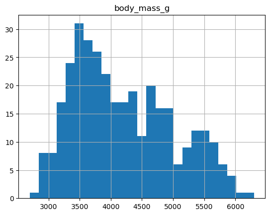
Let’s say we’re interested in the mean boddy mass per species. With two one-liners, we can find the average body mass and plot corresponding histograms (pandas.DataFrame.groupby(), pandas.DataFrame.hist()):

print(pengs.groupby("species")["body_mass_g"].mean())

species
Adelie       3700.662252
Chinstrap    3733.088235
Gentoo       5076.016260
Name: body_mass_g, dtype: float64

pengs.hist(column='body_mass_g', bins=25)

array([[<AxesSubplot:title={'center':'body_mass_g'}>]], dtype=object)

groupby is a powerful method which splits a dataframe and aggregates data in groups. We start by creating a new column child to indicate whether a pengouin was a child or not, based on the existing body_mass_g column. For this example, let’s assume that you are a child when you weight less than 4500 g:

pengs["child"] = pengs["body_mass_g"] < 4000

Now we can test the if the flipper length is different for childs by grouping the data on species and then creating further sub-groups based on child:

pengs.groupby(["species", "child"])["flipper_length_mm"].mean()

species    child
Adelie     False    195.282051
           True     188.098214
Chinstrap  False    203.062500
           True     193.596154
Gentoo     False    217.262295
           True     208.000000
Name: flipper_length_mm, dtype: float64

Each column of a dataframe is a pandas.Series object - a dataframe is thus a collection of series:

# print some information about the columns
pengs.info()

<class 'pandas.core.frame.DataFrame'>
RangeIndex: 344 entries, 0 to 343
Data columns (total 8 columns):
 #   Column             Non-Null Count  Dtype  
---  ------             --------------  -----  
 0   species            344 non-null    object 
 1   island             344 non-null    object 
 2   bill_length_mm     342 non-null    float64
 3   bill_depth_mm      342 non-null    float64
 4   flipper_length_mm  342 non-null    float64
 5   body_mass_g        342 non-null    float64
 6   sex                333 non-null    object 
 7   child              344 non-null    bool   
dtypes: bool(1), float64(4), object(3)
memory usage: 19.3+ KB

Now we can already see what columns are present in the df. Any easier way jsut to display the column names is to use the function df.columns.

pengs.columns

Index(['species', 'island', 'bill_length_mm', 'bill_depth_mm',
       'flipper_length_mm', 'body_mass_g', 'sex', 'child'],
      dtype='object')

Unlike a NumPy array, a dataframe can combine multiple data types, such as numbers and text, but the data in each column is of the same type. So we say a column is of type int64 or of type object.

Let’s inspect one column of the penguin data (first downloading and reading the datafile into a dataframe if needed, see above):

pengs["flipper_length_mm"]
pengs.flipper_length_mm          # same as above

    181.0
    186.0
    195.0
      NaN
    193.0
       ...  
    NaN
  215.0
  222.0
  212.0
  213.0
Name: flipper_length_mm, Length: 344, dtype: float64

A single column of a data frame is often refered to as a "Series".

Now let us adress not just a single column, but also include the rows as well. Adressing a row with numbers is what Pandas calls the index:

pengs.index

RangeIndex(start=0, stop=344, step=1)

We saw above how to select a single column, but there are many ways of selecting (and setting) single or multiple rows, columns and values. We can refer to columns and rows either by number or by their name (loc, iloc, at, iat):

pengs.loc[0,"island"]          # select single value by row and column
pengs.loc[:10,"bill_length_mm":"body_mass_g"]  # slice the dataframe by row and column *names*
pengs.iloc[0:2,3:6]                      # same slice as above by row and column *numbers*

pengs.at[0,"flipper_length_mm"] = 42      # set single value by row and column *name* (fast)
pengs.at[0,"species"]           # select single value by row and column *name* (fast)
pengs.iat[0,5]                           # select same value by row and column *number* (fast)

pengs["is_animal"] = True             # set a whole column

Dataframes also support boolean indexing, just like we saw for numpy arrays:

idx_big = pengs["body_mass_g"] > 4500 
pengs[idx_big]

	species	island	bill_length_mm	bill_depth_mm	flipper_length_mm	body_mass_g	sex	child	is_animal
7	Adelie	Torgersen	39.2	19.6	195.0	4675.0	Male	False	True
39	Adelie	Dream	39.8	19.1	184.0	4650.0	Male	False	True
45	Adelie	Dream	39.6	18.8	190.0	4600.0	Male	False	True
81	Adelie	Torgersen	42.9	17.6	196.0	4700.0	Male	False	True
101	Adelie	Biscoe	41.0	20.0	203.0	4725.0	Male	False	True
...	...	...	...	...	...	...	...	...	...
338	Gentoo	Biscoe	47.2	13.7	214.0	4925.0	Female	False	True
340	Gentoo	Biscoe	46.8	14.3	215.0	4850.0	Female	False	True
341	Gentoo	Biscoe	50.4	15.7	222.0	5750.0	Male	False	True
342	Gentoo	Biscoe	45.2	14.8	212.0	5200.0	Female	False	True
343	Gentoo	Biscoe	49.9	16.1	213.0	5400.0	Male	False	True

115 rows × 9 columns

Using the boolean index idx_big, we can select specific row from an entire df based on values from a single column.

Task 1.8: How many pengouins per species live on which island? Store the answer in a new variable. (2 points).

Task 1.9: Using boolean indexing, compute the mean flipper length among pengouins over and under the average body mass. (2 points).

Tidy data#

The above analysis was rather straightforward thanks to the fact that the dataset is tidy.

In short, columns should be variables and rows should be measurements, and adding measurements (rows) should then not require any changes to code that reads the data.

What would untidy data look like? Here’s an example from some run time statistics from a 1500 m running event:

runners = pd.DataFrame([
            {'Runner': 'Runner 1', 400: 64, 800: 128, 1200: 192, 1500: 240},
            {'Runner': 'Runner 2', 400: 80, 800: 160, 1200: 240, 1500: 300},
            {'Runner': 'Runner 3', 400: 96, 800: 192, 1200: 288, 1500: 360},
            ])

runners.head()

	Runner	400	800	1200	1500
0	Runner 1	64	128	192	240
1	Runner 2	80	160	240	300
2	Runner 3	96	192	288	360

runners = pd.melt(runners, id_vars="Runner",
            value_vars=[400, 800, 1200, 1500],
            var_name="distance",
            value_name="time"
            )

runners.head()

	Runner	distance	time
0	Runner 1	400	64
1	Runner 2	400	80
2	Runner 3	400	96
3	Runner 1	800	128
4	Runner 2	800	160

In this form it’s easier to filter, group, join and aggregate the data, and it’s also easier to model relationships between variables.

The opposite of melting is to pivot data, which can be useful to view data in different ways as we’ll see below.

For a detailed exposition of data tidying, have a look at this article.

Creating dataframes from scratch#

We saw above how one can read in data into a dataframe using the read_csv() function. Pandas also understands multiple other formats, for example using read_excel, read_json, etc. (and corresponding methods to write to file: to_csv, to_excel, to_json, etc.)

But sometimes you would want to create a dataframe from scratch. Also this can be done in multiple ways, for example starting with a numpy array (see DataFrame docs

Let’s create a df for our study and fill it with random numbers which do not make any sense at all.

import random
import string

n = 6

ids = [''.join(random.choices(string.ascii_uppercase + string.digits, k=5)) for i in range(0,n)] # this line generates IDs from Uppercase letters A-Z and Number 0-9 of length 5

nms_cols = ['age','height','MoCA']
rand_age = np.random.randint(18,99,n)
rand_height = np.random.randint(150,200,n)
rand_moca = np.random.randint(0,30,n)
df = pd.DataFrame(list(zip(rand_age, rand_height, rand_moca)), index=ids, columns=nms_cols)
df.head()

	age	height	MoCA
W6YCR	96	170	29
V7W9X	50	189	25
0IY04	41	190	18
2JTTH	22	189	15
O71H4	84	199	15

Data science in practice

s01: Pandas

Contents

s01: Pandas#

Objectives of this session:#

What’s in a dataframe?#

Tidy data#

Creating dataframes from scratch#